
Benchmark Best Practices, part 2. This series collects the checks I apply before I trust a benchmark, whether it comes from a vendor, an internal team or my own test rig. Part 1 covered Amdahl’s law and parallel scaling claims. Part 2 covers Little’s law and the consistency of throughput, latency and concurrency. Further parts will follow.
A benchmark report usually carries three numbers: a throughput, a latency and some measure of concurrency. They are not independent. If the system is stable and the three were measured over the same interval, Little’s law binds them together. When they do not reconcile, the report combined metrics from different boundaries, different populations or different time windows, and I stop reading the conclusions until I know which.
What Little’s law says
Little’s law states L = λ × W. In a stable system, over a defined observation interval, the average number of items in the system (L) equals the average arrival rate (λ) multiplied by the average time each item spends inside the boundary (W).
John D. C. Little published the proof in 1961 as A Proof for the Queuing Formula: L = lambda W. It holds for any boundary you care to draw, which is what makes it useful for review: it applies to a thread pool, a database, a Kafka consumer group or the whole platform, provided you keep the same boundary for all three numbers.
If a service completes 2,000 requests per second at an average residence time of 50 ms, the implied average population is 2,000 x 0.050 = 100 requests. Those 100 requests must exist somewhere inside the chosen boundary at any given moment.
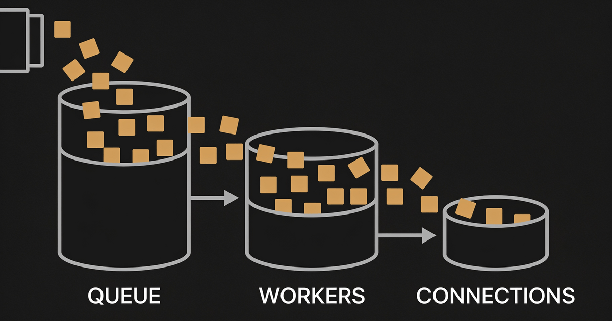
Layered storage benchmarks practice the same discipline. The Ceph performance guide on YourcmcWiki runs three separate test campaigns before it says anything about the whole system: fio on the bare drives, fio through RBD on the cluster, and sockperf on the network. Each campaign owns its own boundary and its own three numbers. Folding them into one storage throughput figure is the mistake this article is about.
| Reported value | Consistency check | What I inspect next |
|---|---|---|
| 2,000 requests per second | Arrival or completion rate, over which interval? | Ramp, steady state and drain phases |
| 50 ms average latency | End to end, or service time only? | Queue time and downstream time |
| 100 requests implied in flight | Does telemetry account for them? | Queues, workers, sockets and retries |
| 20 application workers | Workers are only one part of the boundary | Waiting requests outside the worker pool |
The load generator sets a hard ceiling
Most benchmark tools run closed loop: a fixed number of virtual clients, each sending one request, waiting for the response, then sending the next. Apply Little’s law to the client side and the ceiling appears: with C clients and no think time, throughput can never exceed C / W.
Twenty clients at 50 ms of response time produce at most 400 requests per second. A report that shows 2,000 requests per second at 50 ms from 20 clients is describing something other than what it says: the latency is service time rather than response time, the concurrency is misreported, or the two numbers come from different intervals.
| Closed-loop clients | Response time | Maximum throughput |
|---|---|---|
| 20 | 5 ms | 4,000 requests per second |
| 20 | 50 ms | 400 requests per second |
| 200 | 50 ms | 4,000 requests per second |
| 200 | 500 ms | 400 requests per second |
The closed loop has a second effect worth naming. When the system stalls, the clients stop sending because they are waiting, so the stall is recorded as a few slow requests rather than as the hundreds of requests that would have arrived during it in production. Gil Tene named this coordinated omission in How NOT to Measure Latency. An open-loop generator, which fires at a fixed arrival rate regardless of responses, shows the queue that builds instead. For a system that will face an arrival rate it does not control, the open-loop result is the honest one, and the report should state which model it used.
The utilization law, a sibling check
Draw the boundary around the servers alone and Little’s law becomes the utilization law: utilization equals throughput multiplied by service time per request, the relation Denning and Buzen set out in 1978 in The Operational Analysis of Queueing Network Models.
At 2,000 requests per second with 5 ms of service time per request, the work amounts to 10 server-seconds every second. On 20 workers that is 50 percent utilization, which is plausible. On 4 workers it is impossible, whatever the report says.
The same arithmetic applies to CPU cores, disk queues and database connections, and it is my fastest way to spot a service time that was measured on a warm cache and then presented as representative.
From benchmark to sizing
The same law runs forwards to size a platform. A target of 10,000 requests per second with a latency budget of 20 ms means about 200 requests in flight on average, before any headroom for bursts. Every pool along the path must be able to hold them: connection pools, worker threads, consumer partitions, database connections, and the sockets and file descriptors behind them.
Each hop has its own L, and the one that cannot hold its share becomes the queue where the latency budget is spent. When I size Kafka, Cassandra, ScyllaDB or PostgreSQL against a real workload, this is the first number I compute, because it turns a latency objective into a concrete concurrency requirement per component.
What Little’s law does not tell you
Little’s law does not say that a larger thread pool fixes saturation, and it does not predict the latency curve near capacity. It holds for long-run averages in a stable system: if the queue is still growing when the measurement window closes, there is no steady state and the relation does not apply.
It also says nothing about the distribution. A mean latency of 50 ms can hide a p99 of two seconds, and the p99 is usually what the service objective is written against.
Queueing behavior, service-time distributions and tail latency need their own models and their own measurements. The law only tells you that the averages must reconcile.
My Little’s law checklist for a benchmark report
The checklist below turns Little’s law into the questions I ask any benchmark report. Each one is arithmetic the published numbers must already satisfy. A failure at this stage invalidates the figures before any interpretation of them becomes interesting or actionable.
- Define the boundary. State whether latency starts at the client, the load generator, the service or the storage layer, and keep the same boundary for throughput and concurrency.
- Use one interval. Throughput, latency and concurrency must be averaged over the same window. Separate warmup, steady state and drain, and never average them together.
- Check stability. A queue that grows during the window means the system was not in steady state; the averages from that window prove nothing.
- Reconcile the three numbers. Multiply throughput by latency and compare with the concurrency the report claims. A gap is a finding.
- Check the load generator’s cap. Closed-loop clients divided by response time is the ceiling. Ask which load model was used and whether coordinated omission was handled.
- Apply the utilization law. Throughput times service time against the worker or core count. Above 100 percent is impossible; near 100 percent explains the tail.
- Report distributions. Mean, p50, p99 and max, with the sample count. A mean alone hides the tail that breaks the service objective.
- Repeat and explain variance. A single best run is an anecdote, not a capacity result.
Read with part 1
Part 1 covers the scaling side of the same review discipline: Amdahl’s law, the Karp-Flatt metric and the Universal Scalability Law. Read the two together for the full filter; the image below points at the first part of the series.
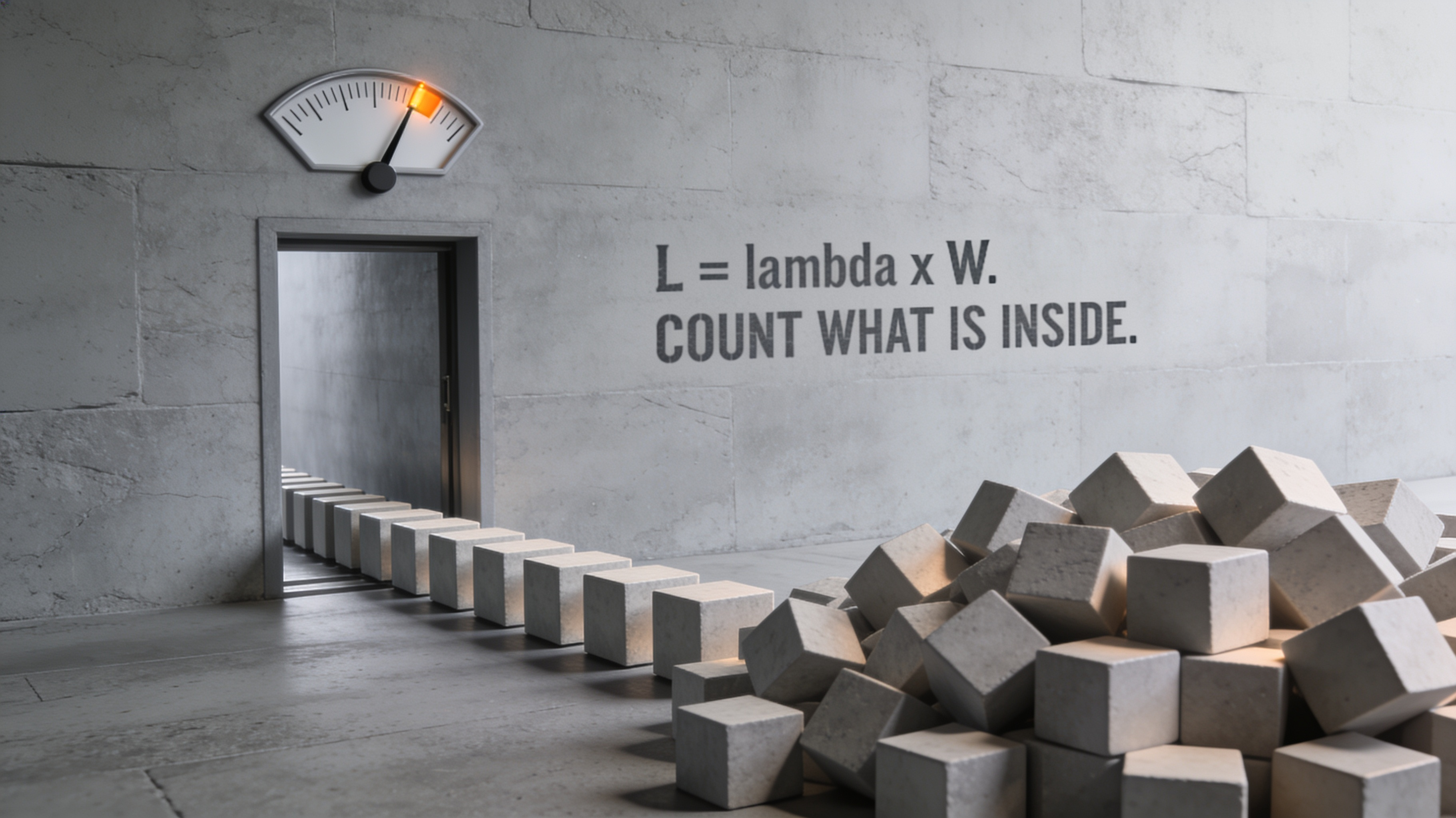
Little’s law tells you when throughput, latency and concurrency describe different systems. It says nothing about whether a parallel speedup claim is reachable at all; that is the job of Amdahl’s law, covered in part 1 of this series. I use both as early filters. If a benchmark survives them, it deserves deeper profiling. If it does not, more hardware will not repair the claim.
If a benchmark is driving a platform purchase or a capacity decision, I can review the workload model, the test method, the bottleneck evidence and the sizing assumptions through a Capacity Planning and Platform Sizing engagement or Data Platform Audit. Book a 15-min intro call to discuss the decision.
Frequently asked questions
What is Little’s law and how does it apply to a benchmark?
Little’s law states that the average number of items in a stable system equals the average arrival rate multiplied by the average time each item spends inside it. Applied to a benchmark, the reported throughput, latency and concurrency must satisfy L = λ × W for one boundary and one observation window. If they do not, the report combined metrics from different boundaries, populations or time windows.
How do I check that throughput, latency and concurrency describe the same system?
Multiply the reported throughput by the reported latency and compare the result with the reported concurrency. The product is the implied in-flight population. Then ask whether the report’s telemetry accounts for that population at the boundary it claims to measure: queues, workers, sockets, retries and downstream calls. A gap is a finding, not a rounding error.
What throughput can a closed-loop load generator actually produce?
A closed-loop generator with C clients and no think time can never have more than C requests in flight, so its throughput is capped at C divided by the response time. Twenty clients at 50 ms of response time produce at most 400 requests per second. If a report shows more, the latency is service time rather than response time, the concurrency is misreported, or the numbers come from different intervals.
What is coordinated omission and why does it hide stalls?
Coordinated omission is the error a closed-loop load generator makes when the system stalls: the clients wait, so they stop sending, and the stall is recorded as a few slow requests instead of the hundreds of requests that would have arrived in production. Gil Tene named it in How NOT to Measure Latency. An open-loop generator, which fires at a fixed arrival rate regardless of responses, shows the queue that builds instead.
What is the utilization law and how do I use it to audit a report?
The utilization law is Little’s law drawn around the servers alone: utilization equals throughput multiplied by service time per request. At 2,000 requests per second with 5 ms of service time, the work is 10 server-seconds every second. On 20 workers that is 50 percent utilization. On 4 workers it is impossible. Above 100 percent is impossible, and near 100 percent explains the tail.
How does Little’s law turn a latency budget into a sizing requirement?
A target of 10,000 requests per second with a 20 ms latency budget implies about 200 requests in flight on average before headroom. Every pool along the path must be able to hold them: connection pools, worker threads, consumer partitions, database connections and the file descriptors behind them. The hop that cannot hold its share becomes the queue where the latency budget is spent.
Sources
- John D. C. Little, A Proof for the Queuing Formula: L = lambda W, 1961.
- Peter J. Denning and Jeffrey P. Buzen, The Operational Analysis of Queueing Network Models, 1978.
- Gil Tene, How NOT to Measure Latency.
- Ceph performance, YourcmcWiki.
Update 2026-09-29. This post is now part of Performance and Cost Engineering for Data Platforms, the field guide to performance and cost engineering.
0 Comments