
Benchmark Best Practices, part 1. This series collects the checks I apply before I trust a benchmark, whether it comes from a vendor, an internal team or my own test rig. Part 1 covers Amdahl’s law and parallel scaling claims. Part 2 covers Little’s law and the consistency of throughput, latency and concurrency. Further parts will follow.
A benchmark is a measurement with a boundary. Change the workload, the cluster size, the dataset, the cache state or the observation window and you have a different result. Before I compare two platforms, I check whether the reported numbers are internally possible. For scaling claims, the first filter is Amdahl’s law. It takes a few minutes with the numbers already in the report and it catches errors that would otherwise cost a week of test runs.
What Amdahl’s law says
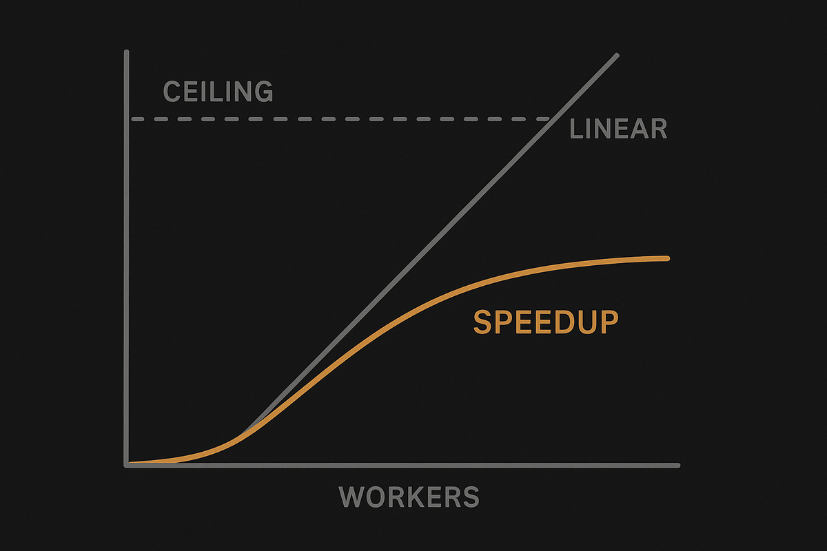
For a fixed workload, Amdahl’s law expresses the speedup from N parallel workers as S(N) = 1 / (s + (1 - s) / N), where s is the fraction of the work that remains serial. Gene Amdahl presented the argument in his 1967 paper, Validity of the Single Processor Approach to Achieving Large Scale Computing Capabilities.
The ceiling is 1 / s. A 10 percent serial fraction caps the theoretical speedup at 10x, however many workers you add. With eight workers the same workload reaches only about 4.71x, because the parallel part is still spread across a finite number of workers.
| Serial fraction | 8 workers | 32 workers | Theoretical ceiling |
|---|---|---|---|
| 20% | 3.33x | 4.44x | 5x |
| 10% | 4.71x | 7.80x | 10x |
| 5% | 5.93x | 12.55x | 20x |
Turn the claim into an implied serial fraction
The most useful review move is to run the law backwards. A report gives you a speedup S on N workers. Solve for the serial fraction that would produce it: s = (1 / S - 1 / N) / (1 - 1 / N).
Karp and Flatt proposed this experimentally determined serial fraction in 1990, in Measuring Parallel Processor Performance. Then ask whether the pipeline described in the report can plausibly contain that little serial work.
| Claimed speedup on 32 workers | Implied serial fraction | What it would require |
|---|---|---|
| 30x | 0.2% | Almost no coordination, shuffle, commit or skew on the critical path |
| 24x | 1.1% | A well partitioned job with light coordination |
| 16x | 3.2% | Typical for a job with a real shuffle or a global aggregation |
| 8x | 9.7% | A significant serial stage or a shared resource near its limit |
Compute it at every cluster size the report provides, not only the largest. If the implied serial fraction is stable across sizes, the fixed-workload model fits and the ceiling is real. If it rises with the worker count, the cost of coordination grows with the cluster: more shuffle connections, more straggler waiting, more metadata traffic, more retries. That is a different problem from a fixed serial stage, and more hardware makes it worse rather than better.
What the Universal Scalability Law adds
Amdahl’s law treats coordination as free. It caps how far a fixed workload can speed up, but it charges nothing for the workers talking to each other. Neil J. Gunther’s Universal Scalability Law closes that gap. It expresses relative capacity as C(N) = N / (1 + α(N - 1) + βN(N - 1)).
Where N is the number of workers, C(N) the throughput relative to one worker, α the contention term and β the coherency term.
The two parameters separate the two ways parallel systems stop scaling. Contention is queueing for resources that cannot be divided, and it plays exactly the role of the serial fraction s in Amdahl’s law. Coherency is the price of keeping distributed state consistent, charged on every exchange between workers, so its cost grows with the N(N – 1) pairs of workers rather than with N alone.
Set β to zero and the USL collapses into Amdahl’s law: capacity rises toward a fixed ceiling of 1/α and flattens there. With β above zero the curve peaks at Nmax = sqrt((1 - α) / β) and then declines. Past that peak, each added worker destroys capacity, something Amdahl’s law can never express. Vendors rarely publish measurements far enough past the peak to show it.
The law earns its keep as a sizing tool. Fit α and β from measurements at four or five sizes and the fitted curve locates the peak before you reach it, which turns a scaling decision into arithmetic instead of hope. The USL calculator on tools.ntsd.dev fits the two parameters from pasted measurements in a browser, and this walkthrough of Gunther’s law on Graphium Labs develops all three regimes, linear, plateau and retrograde, with worked examples. My own spreadsheets for client engagements follow the same recipe.
Where adding vCPUs per image destroyed global throughput
This regime is not hypothetical. The measurements come from the preproduction environment of an image processing platform. Each point assigns more vCPUs to a single image while keeping the workload identical, from 7 to 241 per image, and global throughput falls at every step.
A second, coarser resolution class produced the identical normalized curve; the chart shows the finer class, whose larger files make it the heavier workload. I keep the client and the absolute figures confidential. Relative numbers carry the full lesson.
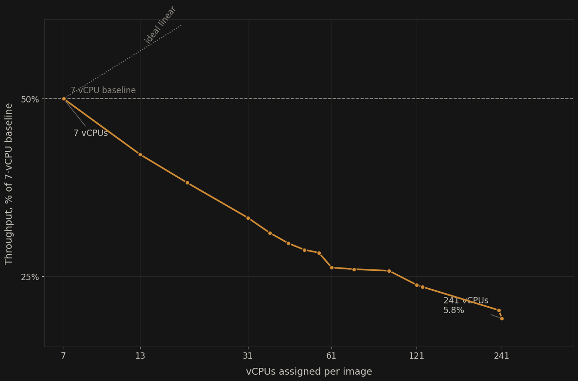
| vCPUs assigned per image | Global throughput, relative to baseline | Efficiency |
|---|---|---|
| 7 | 100% (baseline) | 100% |
| 13 | 48% | 26% |
| 31 | 21% | 4.8% |
| 61 | 11% | 1.3% |
| 121 | 8.9% | 0.52% |
| 241 | 5.8% | 0.17% |
Run the implied serial fraction across the same series. Between allocations of 7 and 13 vCPUs per image it already exceeds 300 percent. It passes 1000 percent by 61 and 1700 percent at 241. Above 100 percent, the fixed-workload model has stopped describing the system: coordinating the added workers costs more than their work contributes.
Fitting the USL to these measurements puts the curve deep in the coherency-dominated regime. The fitted peak sits below the smallest tested allocation, and the fitted curve keeps falling beyond the last measurement, through the larger allocation the team was evaluating.
The remediation follows from the shape of the curve rather than from any single component. If hardware becomes the limitation in production, giving each image fewer vCPUs raises global throughput on the same machines. Per-image allocation, not another hardware order, is the knob that protects total capacity.
That is why I compute the implied serial fraction before anything else in a scaling report. When it climbs past 100 percent, no further benchmark run will rescue the claim, and the next hardware order makes the result worse, not better.
Where the serial fraction hides in a data platform
In a data platform the serial fraction rarely looks like a single-threaded loop. It hides in a coordinator, a metadata lock, a commit barrier, a global aggregation, a skewed partition that one worker owns, or a single output sink. The useful question is not whether the storage or the network looks busy. It is which part of the critical path cannot progress in parallel, and how long that part takes on its own.
Amdahl’s law is a bound, not a diagnosis. It tells you that a serial fraction exists and how large it must be. Finding it takes profiling and stage timing. If a benchmark scales the workload with the cluster, changes the algorithm or removes work entirely, the fixed-workload model no longer describes the experiment. State that change instead of claiming that the law was beaten.
Big Data: capacity scaling is not speedup
Big Data workloads make the gap between available parallelism and useful scaling easy to see. A Spark, Flink or distributed SQL job can divide billions of records across workers, but scheduling, metadata access, shuffle coordination, skewed partitions, global aggregation and the final commit still constrain the critical path. Linear scaling is the ideal upper bound. In production it is rarely reached across a wide range of cluster sizes.
Sometimes adding workers produces almost no speedup. A stage can be limited by memory bandwidth, shared storage throughput, network capacity, a single reducer or a partition that holds most of the data. Extra executors then add CPU and memory without dividing the resource that controls elapsed time. The scaling curve flattens even when cluster utilization looks busy.
Memory capacity creates another case that benchmark reports often hide. The dataset or the working set may not fit on one worker, or even on a small cluster. The job fails, spills so heavily that it enters a different operating regime, or exceeds the maximum test duration. In that situation there is no valid small-cluster baseline for the fixed workload. The additional workers make the problem feasible. That is capacity scaling, not evidence of linear speedup.
| Observed behavior | Likely interpretation | How to report it |
|---|---|---|
| Runtime falls, but less than the worker count rises | Serial work, coordination, skew or a shared resource limits strong scaling | Report speedup and efficiency from the same fixed dataset |
| Runtime barely changes after adding workers | The limiting resource is not divided by the new workers | Measure memory, network, storage and hottest-partition throughput |
| The job cannot run on the smaller cluster | The comparison starts below the minimum capacity the workload needs | Start strong-scaling results at the smallest feasible cluster |
| Dataset size grows with the worker count while runtime stays stable | The test measures weak scaling rather than fixed-workload speedup | Report data per worker and label the test as weak scaling |
Weak scaling has its own law. John Gustafson argued in 1988, in Reevaluating Amdahl’s Law, that when the problem grows with the machine, scaled speedup can stay close to linear. Both laws are correct. They answer different questions. The misleading move is to measure weak scaling and report it in the language of fixed-workload speedup.
For a Big Data benchmark I therefore publish two separate results. Strong scaling asks how much faster the same dataset runs, starting with the smallest cluster that can execute it credibly. Weak scaling asks how much more data the platform can process as resources grow. Combining the two can make a platform look linear when the fixed workload did not speed up at all.
My Amdahl checklist for a benchmark report
The checklist below is the short form I run on any benchmark report before its numbers enter a decision. Each item is a question the report must already answer; anything missing is asked before the profiling work has started, never after.
- Fix the workload. Same dataset, same request mix, same key distribution, same configuration at every cluster size. Anything that changed with the size is a second experiment.
- Start at a credible baseline. The smallest cluster that runs the fixed workload without spilling into a different regime or failing. A baseline that cannot hold the working set inflates every ratio above it.
- Report speedup and efficiency. Efficiency is speedup divided by the worker count. A 12x result on 32 workers is 37.5 percent efficiency, and the report should say so.
- Compute the implied serial fraction at every size. Stable means a real ceiling. Rising means coordination cost that grows with the cluster. Past 100 percent the platform loses more capacity than the added workers contribute; stop growing and profile what they all share.
- Name the serial components. Coordinator, barrier, commit, global aggregation, skewed partition, single sink. Time each one on its own.
- Separate strong from weak scaling. Two results, two labels, never one blended curve.
- State what changed when the law appears beaten. A different algorithm, a cache that fits, removed work. Superlinear results have a cause, and the cause is the finding.
Next in the series
Amdahl’s law tells you when a scaling promise exceeds the fixed-workload ceiling. It says nothing about whether the throughput and latency figures in the same report describe the same system. That is the job of Little’s law, and it is the subject of part 2 of this series. I use both as early filters. If a benchmark survives them, it deserves deeper profiling. If it does not, more hardware will not repair the claim.
If a benchmark is driving a platform purchase or a capacity decision, I can review the workload model, the test method, the bottleneck evidence and the sizing assumptions through a Capacity Planning engagement or Data Platform Audit. Book a 15-min intro call to discuss the decision.
Frequently asked questions
What is Amdahl’s law?
Amdahl’s law bounds the speedup a fixed workload can get from parallel workers. With N workers and a serial fraction s, the speedup is S(N) = 1 / (s + (1 – s) / N), and the ceiling as N grows without limit is 1 / s. A workload that is 10 percent serial cannot exceed 10x however many workers you add, and it reaches only about 4.71x on eight. Gene Amdahl published the argument in 1967.
How do I check a vendor’s parallel scaling claim?
Run the law backwards. Take the claimed speedup S on N workers and solve for the serial fraction that would produce it: s = (1 / S – 1 / N) / (1 – 1 / N). Karp and Flatt proposed this experimentally determined serial fraction in 1990. Then ask whether the pipeline described in the report can plausibly contain that little serial work. A claim of 30x on 32 workers implies 0.2 percent serial, which means almost no coordination, shuffle, commit or skew anywhere on the critical path.
What is the difference between Amdahl’s law and Gustafson’s law?
They answer different questions and both are correct. Amdahl’s law fixes the workload and asks how much faster it runs on more workers, which is strong scaling. John Gustafson argued in 1988 that when the problem grows with the machine, scaled speedup can stay close to linear, which is weak scaling. The misleading move is to measure weak scaling and report it in the language of fixed-workload speedup.
What is the Universal Scalability Law and when do I need it?
Amdahl’s law treats coordination as free: it caps speedup but charges nothing for workers talking to each other. Neil Gunther’s Universal Scalability Law adds that cost as C(N) = N / (1 + α(N – 1) + βN(N – 1)), where α is the contention term and β the coherency term. You need it whenever throughput falls rather than merely flattens as you add workers, because the coherency term is the only one of the two that produces a retrograde curve. Fit α and β from four or five measured sizes and the fitted curve locates the peak before you reach it.
Why did my pipeline get slower after I gave it more CPUs?
Because per-worker allocation and global throughput are different quantities, and coordination cost can exceed the work the added CPUs contribute. On the image processing pipeline in this article, raising the allocation from 7 to 241 vCPUs per image took global throughput from 100 percent of baseline down to 5.8 percent, on the same hardware and the same workload. The implied serial fraction passed 100 percent between the first two points, which is the signal that the fixed-workload model has stopped describing the system. The fix was to give each image fewer vCPUs, not to buy more hardware.
What is the difference between strong scaling and weak scaling?
Strong scaling holds the dataset fixed and asks how much faster it runs as the cluster grows. Weak scaling grows the dataset with the cluster and asks how much more data the platform can process. A Big Data benchmark should publish both as separate labeled results, with strong scaling starting at the smallest cluster that runs the workload credibly. Blending them makes a platform look linear when the fixed workload did not speed up at all.
If a benchmark is driving a platform purchase or a capacity decision, I can review the workload model, the test method, the bottleneck evidence and the sizing assumptions through the Capacity Planning and Platform Sizing engagement. Book a 15-min intro call to discuss the decision.
Update 2026-09-29. This post is now part of Performance and Cost Engineering for Data Platforms, the field guide to performance and cost engineering.
0 Comments