Download this article (PDF) 621 KB

A format comparison needs an object-count column alongside its byte-count column. Compression changes the stored payload; packaging determines how many keys, uploads and metadata records the application creates. The two can move independently. A compact dataset can still be expensive to ingest, discover or clean up when it becomes a large population of small objects.
I would measure the reader as well as the writer before choosing a layout. Consolidating tiles into fewer objects can reduce the object population while leaving many range requests on the read path. The useful comparison is the complete workflow, with its request mix and update behavior, rather than the smallest file or the smallest object count alone.
Revised October 21, 2026. This version replaces a private workload comparison with an explicit synthetic example, corrects the distinction between point-cloud formats, and removes assumptions that requests, bills or maintenance times scale exactly with object count. No customer data or environment details are included.
Compression and packaging answer different questions
Compression measures the bytes needed to represent data, while packaging determines the objects that hold that representation. A comparison of formats should record both. Matching the source dataset does not guarantee identical output bytes: indexes, hierarchy information, attributes, precision and encoding can differ. The object count only becomes meaningful alongside those settings and the intended reader.
| Comparison axis | What to record | What it does not establish |
|---|---|---|
| Stored bytes | Payload, indexes, metadata files and retained versions | The number of requests or the latency of an interactive read |
| Object population | Data keys, hierarchy keys, manifests and other persisted artifacts | A fixed request count or backend allocation multiplier |
| Application access | Requests, transferred bytes, cache behavior and decode work per useful result | The cost of future updates, retries or cleanup |
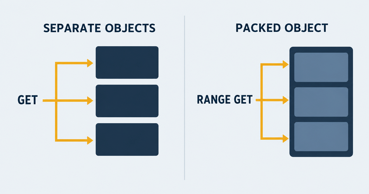
This matters for point clouds, but also for image tiles, training shards and analytical files. A logical tile or chunk does not have to become a separate object. A container can preserve internal spatial partitions and let a reader fetch selected byte ranges, provided the index, client and serving path support that access.
Point-cloud formats do not share one layout
PotreeConverter, EPT and COPC organize point-cloud data differently, so their output counts should not be grouped under one rule. Count the files produced by the selected converter release and the keys actually uploaded. Include hierarchy and metadata artifacts, and check whether a publishing pipeline splits, bundles or duplicates them before they reach object storage.
| Format or converter | Documented organization | What to verify |
|---|---|---|
| PotreeConverter 2.0 | The project describes three output files, contrasting with the per-node files of 1.7. | Actual release, generated artifacts, upload mapping and reader compatibility |
| Entwine Point Tile (EPT) | Separate point-data files, hierarchy files and JSON metadata | Count every artifact class; node count alone misses supporting files. |
| Cloud Optimized Point Cloud (COPC) 1.0 | Spatially organized chunks and hierarchy within a single LAZ file | Range access, index reads, caching and the number of files used for the full collection |
These distinctions come from the PotreeConverter documentation, the EPT format description and the COPC specification. A single COPC file is not a promise that an entire collection fits in one object, or that a view requires only one GET.
A synthetic example isolates the object-count effect
Holding encoded payload volume constant isolates the arithmetic of packaging. In this example, 100 GiB divided into uniform 64 KiB objects requires 1,638,400 objects; divided into 16 MiB objects, it requires 6,400. That is a 256-fold count difference, before indexes and metadata. It is a calculation, not a point-cloud benchmark or a customer result.
| Uniform payload per object | Objects in 100 GiB | Successful writes if one PUT per object |
|---|---|---|
| 64 KiB | 1,638,400 | 1,638,400 |
| 1 MiB | 102,400 | 102,400 |
| 16 MiB | 6,400 | 6,400 |
The rightmost column is valid because the example specifies the upload method. It does not predict a 256-fold bill, a 256-fold speedup or a 256-fold reduction in scan duration. Those outcomes depend on other work and on how the service and client process it.
One object does not mean one request
Object count and API request count are related through the operations an application performs. A single upload can use multipart calls, a reader can request several ranges from one object, and a listing can return many keys. Retries, validation and caching add further differences. Count operations from the client or service rather than infer them from a file inventory.
Amazon S3’s multipart upload process has initiation, part uploads and completion. An illustrative upload of eight parts therefore uses ten successful calls before any additional validation or retries. It produces one completed object, not ten.
The GetObject API supports a byte range, but not multiple separate ranges in one GET. A reader may issue several requests for hierarchy and data inside one container, or fetch a wider range to reduce request count at the cost of extra transferred bytes. Check the client’s behavior through the actual proxy or CDN, not just against a local file.
Other operations batch work: ListObjectsV2 returns up to 1,000 objects per request, while DeleteObjects accepts up to 1,000 keys or version references. Listing, deletion and single-object reads do not share a one-key-per-request model. Inspect per-item deletion results and versioning semantics before treating cleanup as complete.
Fewer objects introduce their own tradeoffs
Consolidation can reduce the number of stored keys while increasing the amount of data a small change must rewrite. It can also change the reader’s cache, index and range-fetch behavior. Choose packaging against the required access and update patterns; the minimum object count is not automatically the best operational layout.
For an interactive viewer, record time to the first useful view, requests during navigation, transferred bytes and decode time. For a batch reader, record useful throughput and read amplification. Compare the same data selection and fidelity so that a faster result does not merely omit work or return less detail.
For updates, measure what must be regenerated, rewritten and invalidated when one region changes. Separate per-object authorization and retention requirements from internal chunk boundaries. Packing several logical records into one object can make independent access, deletion or retention harder to implement.

Measure cost and cleanup on the actual backend
The cost of an object population depends on the service and deployment. A managed service may charge for requests and retrievals; a self-hosted store may instead expose the cost through metadata, device operations and maintenance work. Neither API compatibility nor object count supplies a universal billing formula or background-scan speed.
For managed storage, apply the relevant operation prices, storage class, region and contract to the measured request mix. For self-hosted storage, measure metadata growth, allocated space and background work on the deployed build. Do not assign a version ID or a fixed physical metadata envelope to every object on every S3-compatible engine.
Cleanup needs ownership of datasets, not just a list of keys. I would give each published dataset a manifest and distinguish incomplete work from objects still referenced by readers. An interrupted conversion can leave data behind, but age alone does not prove an object is orphaned. Test candidate selection without deletion first, protect active jobs, and handle retained versions and incomplete multipart uploads explicitly.
The object-storage sizing guide covers the broader capacity model. The MinIO small-file analysis and MinIO/XFS guide examine particular backends; their mechanisms are not API-wide constants.
What should a format benchmark record?
A useful format benchmark records the complete published output and a representative read, update and cleanup workload. I would keep compression, object population and API activity as separate columns, then assess their combined operational cost. The benchmark should preserve enough configuration detail to explain why a result changes when the format, client or backend changes.
- Fix the source selection, attributes, precision and required output fidelity. Record converter, reader and storage versions.
- Count every published artifact and its size. Separate data, hierarchy, manifests, versions and temporary output.
- Capture actual PUT, part-upload, GET, HEAD and LIST activity, including retries. Time conversion and upload separately.
- Run cold and warm reads with the real viewer or consumer. Record useful-result latency, transferred bytes and decode work.
- Exercise a bounded update and an interrupted job. Verify publication consistency and cleanup candidates before any deletion.
FAQ
Object count is a useful capacity and workload input, but it does not replace measurement of requests or reader behavior. A format’s logical partitions, its physical files and the uploaded keys may differ. The answers below keep those units separate so that a packaging comparison does not become an unsupported performance claim.
Does better compression reduce object count?
Not necessarily. Compression changes bytes; the writer’s packaging and partitioning determine the object population. Count the actual uploaded keys, including supporting metadata, instead of inferring count from compression ratio.
Does one COPC file require one GET?
No. A range-capable reader can request hierarchy and data chunks separately within the same file. Request count depends on the reader, selected region, caching and serving path. File consolidation alone does not establish a read-request reduction.
Do fewer objects guarantee a proportional saving?
No. Savings depend on the operation mix, pricing, backend allocation and time spent doing useful work. A synthetic single-PUT example can predict those writes, but not the complete bill, scan duration or application speedup.
Should a dataset use the largest possible objects?
Not by default. Larger containers can change range-read efficiency, update cost, access boundaries and independent deletion. Test the required reads and updates before choosing the packaging unit.
Related object-storage guides
This article focuses on how a producer’s format choices become an object-storage workload. The linked guides cover the broader sizing model and backend-specific investigations. Use them to identify what to test, then verify release-sensitive details on the actual platform rather than transfer a numerical example between engines.
- Object storage for data platforms at scale
- Small-file overhead in erasure-coded MinIO
- MinIO and lots of small files
- MinIO/XFS inode accounting and prefix design
- HDD cost and operational tradeoffs in MinIO
Primary format and API sources are linked next to the relevant claims and were checked on October 21, 2026. No vendor endorsement is implied. Numerical examples are original calculations, not production benchmark results.
If a pipeline’s output format is driving a storage decision, I can review the workload and sizing assumptions through a Capacity Planning and Platform Sizing engagement. For an existing system, see the data platform audit, or book a free 15-minute intro call to discuss the decision.
0 Comments